Rangelands, savannas & native grasslands

About the NCMC

The Natural Capital Measurement Catalogue (NCMC) is an open resource that presents metrics and methods for the measurement of natural capital assets, flows of services or benefits, and organisational impacts or dependencies on nature.

The NCMC was designed to help facilitate the integration of natural capital considerations into business, financial and government decision-making, by addressing the need for convergence around a common language and a core set of natural capital metrics.

When businesses incorporate natural capital into their decision-making, it creates space for improvements in a range of areas, such as supply-chain management, risk assessment and management, business sustainability, resilience, and uninterrupted production and operation.

Governments can use information on the state of natural capital to provide important practical information for evaluating different policies, investment objectives and financial risk management.

The NCMC supports business and government to measure – and consequently manage – their natural capital assets, flows of services or benefits, and organisational impacts or dependencies on nature.

This digital iteration of the open reference NCMC is intended to demonstrate a possible new arrangement, plus some further extensions, of natural capital measures found in the proof of concept, which was enabled by the support of NAB. Current development was made possible thanks to the support of the Macdoch Foundation.

Please consider if the metrics and methods you select are relevant to your context and purpose.

We welcome your ongoing feedback to develop the NCMC. Please feel free to explore the Help and Glossary, or leave us a note in the feedback section below.

Please scroll down for Frequently Asked Questions, Glossary of Terms and References.

Frequently Asked Questions

How can I use the NCMC?

The NCMC supports business and government to measure – and consequently manage – their natural capital assets, flows of services or benefits, and organisational impacts or dependencies on nature.

Users can consult the NCMC to identify metrics that they can use in:

management of natural capital assets (e.g. at the farm level of corporate value chains or within defined, managed land areas)

management of an organisation’s nature-related risks and opportunities (e.g. indirectly through supply chains or directly through business operations)

or external reporting (e.g. against disclosure standards and frameworks).

Methods, guidance, references and data sources are provided for each metric, where available.

If entities are unsure of where to begin measuring their natural capital, the NCMC presents three ‘tiers’ of metrics and methods.

This allows unfamiliar users to get started on their natural capital measurement journey, taking into account the user’s needs, resources and deadlines.

For more help navigating your overall approach to natural capital accounting or natural capital assessment, we recommend accessing CSIRO’s Natural Capital Handbook.

Which international standards and frameworks can the NCMC help me report to?

The NCMC is designed to present natural capital accounting and assessment metrics that are consistent with national and international standards and frameworks such as the United Nations System of Economic-Environmental Accounting (SEEA) and the Taskforce on Nature-related Financial Disclosures (TNFD).

How is the NCMC being developed?

The NCMC was developed by Climateworks Centre in partnership with a broad range of stakeholders across Australia working in the natural capital space – including land managers, financial institutions, measurement providers, government, consultancy, research and supply chains organisations.

The ongoing technical development of the NCMC is governed by a group of technical experts from CSIRO, ANU, La Trobe University, Griffith University, Federation University, Accounting for Nature and Farming for the Future. These experts have an active interest in advancing the measurement and management of natural capital in Australia and globally.

The development of the NCMC is made possible through the support of the Macdoch Foundation.

What are the relationships between natural capital accounting and natural capital assessment?

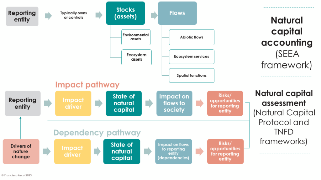
This diagram illustrates some important relationships between natural capital accounting and natural capital assessment.

The main focus of natural capital accounting is on natural assets, and the flows of benefits derived from those assets (although it is acknowledged that the SEEA framework also includes various other items, such as environmental activity accounts that record expenditures on environmental protection and resource management). When applied at a country level, the scope is defined by territorial boundaries, whereas when applied at the level of an individual entity, the scope would normally be defined by the entity’s ownership or control.

Natural capital assessment considers the reporting entity’s impacts and dependencies on natural capital through the concept of impact and dependency pathways, and may involve any natural capital causally related to the entity through these pathways, regardless of territory, ownership or control. Both pathways involve changes to the state of natural capital (equivalent to accounting for stocks of natural assets) and changes to flows (equivalent to accounting for flows of benefits from natural assets), but are differentiated according to the principal cause and effect of these changes.

Impacts involve changes caused by the reporting entity, which may ultimately result in consequences for the reporting entity (such as increased regulation, fines or loss of access to certain markets).

In the case of dependencies, changes are typically caused by wider change drivers (such as climate change) which may ultimately result in consequences for the reporting entity due to changes in the availability of flows that the entity depends or relies on.

Importantly, it is not always necessary to fully account for changes in the state of natural capital, or the availability of flows, in order to characterise an entity’s impacts or dependencies. For example, information on an entity’s greenhouse gas emissions (an impact driver) may be sufficient, without also providing a full account of the state of greenhouse gases in the atmosphere. Likewise, information on the availability of essential flows to a reporting entity may be sufficient, without also providing a full account of the state of the natural capital asset(s) that provide those flows (particularly when the natural capital assets in question are now owned or controlled by the reporting entity, it may be unreasonable to expect them to provide such information).

For more help navigating your overall approach to natural capital accounting or natural capital assessment, we recommend accessing CSIRO’s Natural Capital Handbook.

What are the Tiers?

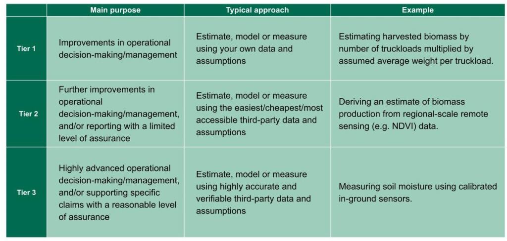
Natural capital can be measured in many different ways, by different users for different purposes. The NCMC allocates metrics and methods to three tiers, corresponding to different user needs and approaches to measurement, as summarised in the table below.

- Verifiability, accuracy and costs tend to increase as you move from Tier 1 to Tier 3.

- Confidence/error tends to shift from unknown to quantified from Tier 1 to Tier 3.

- Ease of use and accessibility generally moves from easy through to challenging from Tier 1 to Tier 3.

What is the difference between 'Environmental Assets' and 'Ecosystem Assets'?

Environmental Assets are measures for natural assets, relatively easily measured as individual components of the environment that provide economic benefits (e.g. mineral resources, land, timber and water). Covered by the SEEA Central Framework (SEEA-CF) and measured in terms of physical quantity and monetary value.

Ecosystem Assets are measures for the sub-set of environmental assets which involve diverse ecosystems. Ecosystem assets are covered by the SEEA Ecosystem Accounting (SEEA-EA) and measured in terms of extent and condition. Produce flows of ecosystem services which can be measured in physical and monetary terms.

Is there a version of the NCMC available as a spreadsheet?

Yes, you can download the spreadsheet version by clicking on the link below:

NCMC_Version1_Spreadsheet_Climateworks

How does NCMC Version 1.0 differ from the Proof of Concept?

Since the release of the proof-of-concept in 2021, the NCMC has been refined and expanded based on expert stakeholder feedback to include updates such as:

broadening of scope to other forms of land use types beyond agriculture
supporting both natural capital accounting and natural capital assessment measures
closer alignment with the United Nations System of Economic-Environmental Accounting (SEEA)
inclusion of natural capital impacts and dependencies, aligned with Taskforce on Nature-related Financial Disclosures (TNFD).
consistency with national and state data and the IUCN Global Ecosystem Typology
ecosystem measures based on ecosystem areas: extent, condition, ecosystem services (physical, monetary)
Consistency with the Natural Capital Protocol and ISSB’s IFRS S1.

Where can I go to access further resources to support my overall natural capital measurement approach?

For more help navigating your overall approach to natural capital accounting or natural capital assessment, we recommend accessing CSIRO’s Natural Capital Handbook.

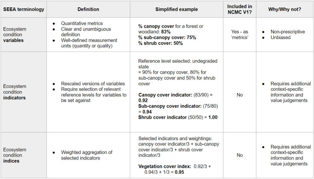
What is a metric vs a variable/indicator/index (SEEA definitions), and how are they included or not in the NCMC?

The following table outlines the SEEA definitions of variable vs indicators vs index (indices) and how they are included or not in the NCMC:

How are metrics, methods and other material selected for the NCMC?

Metric inclusion guidelines

A ‘metric’ in the NCMC is something you can measure that tells you something useful about nature. Official definitions include a “system or standard of measurement”¹ or “a set of figures or statistics that measure results”²,.

The metric should be applicable* to a broad range of end users and purposes.
The metric should be a variable (see SEEA definition)
Where possible, the metric must be practical and achievable to measure.
Where possible, the metric aligns to an internationally and/or nationally recognized standard or framework (e.g. UN SEEA or TNFD).

Method inclusion guidelines

A ‘method’ is “a particular procedure for accomplishing or approaching something, especially a systematic or established one”³. In the NCMC, a method is a particular procedure for measuring a metric. The method can be solely for a specific metric, or part of a suite of procedures for different metrics.

The method should be applicable* to a broad range of end users and purposes.
Where possible, the method should be practical and achievable to measure.
The method should be scientifically credible, based on robust evidence and/or widely accepted.
Priority will be given to:
Methods developed in the Australian context
Internationally recognised methods
The method should be open-access.

Reference material and data sources inclusion guidelines

Reference materials are sources of information, e.g. cited publications.

Data sources are sources of data, e.g. databases.

The reference material/data source should be open-access and/or widely used or referenced.
Reference material/data sources should be able to prove scientific credibility, based on evidence, research and/or strict governance guidelines.
Priority will be given to reference materials/data sources that are:
1. Developed in the Australian context
2. Internationally recognised

*language of original metric/method may be adapted to ensure generic applicability to a broad range of users.

¹TNFD, 2023, Oxford English Dictionary

²,³ Oxford English Dictionary

Glossary of terms

Abiotic flows: "abiotic flows are contributions to benefits from the environment that are not underpinned by or reliant on ecological characteristics and processes"
_{Source/reference: SEEA-EA 2021, para. 6.35.}
_{Note: The monetary value of abiotic flows should not be included in the calculation of the value of ecosystem assets, but reported separately using market prices (SEEA-EA, s. 6.4.5).}

Asset: "a store of value representing a benefit or series of benefits accruing to an economic owner by holding or using the entity over a period of time. It is a means of carrying forward value from one accounting period to another."
_{Source/reference: SEEA-CF 2014, para. 5.32.}

Benefits: "Benefits are the goods and services that are ultimately used and enjoyed by people and society"
_{Source/reference: SEEA-EA 2021, para. 6.16.}

Carbon Sequestration: The removal of carbon dioxide from the atmosphere.

Carbon retention: The storage of sequestered carbon.

Cultural Services: "Cultural services are the experiential and intangible services related to the perceived or actual qualities of ecosystems whose existence and functioning contributes to a range of cultural benefits"
_{Source/reference: SEEA-EA 2021, para. 6.51.}

Dependency/Dependencies on nature: "Dependencies are aspects of environmental assets and ecosystem services that a person or an organisation relies on to function. A company’s business model, for example, may be dependent on the ecosystem services of water flow, water quality regulation and the regulation of hazards like fires and floods; provision of suitable habitat for pollinators, who in turn provide a service directly to economies; and carbon sequestration."
_{Source/reference: TNFD (2023, p. 115)}
_{Note: See also: Natural Capital Protocol definition of a natural capital dependency as a “business reliance on or use of natural capital” (Natural Capital Coalition, 2016, pp. 16-17).}

Disease: "A disorder of structure or function in a human, animal, or plant, especially one that produces specific symptoms or that affects a specific location and is not simply a direct result of physical injury."
_{Source/reference: Oxford English Dictionary.}

Disturbed area: "A clearly defined geographical space that has been subject to human activity that has changed the land’s surface condition, relative to a reference state."
_{Source/reference: TNFD (2023, p. 116).}

Drivers of nature change: "All external factors that affect nature, anthropogenic assets, nature’s contributions to people and good quality of life. They include institutions and governance systems and other indirect and direct drivers (both natural and anthropogenic)."
_{Source/reference: TNFD (2023, p. 116)}

_{Note: See also: Drivers of nature change include: climate change; land/freshwater/ocean use change; resource use/replenishment; pollution/pollution removal; and invasive alien species introduction/removal (TNFD 2023, p. 30).}

Ecosystem: "An ecosystem is a dynamic complex of plant, animal and micro-organism communities and their non-living environment interacting as a functional unit"
_{Source/reference: SEEA-EA, para. 2.6.}

Ecosystem accounting area (EEA): "the geographical territory for which an ecosystem account is compiled."
_{Source/reference: SEEA-EA 2021, para. 2.12.}

Ecosystem asset: "ecosystem assets are contiguous spaces of a specific ecosystem type characterized by a distinct set of biotic and abiotic components and their interactions."
_{Source/reference: SEEA-EA 2021, para. 2.11.}
_{Note: Ecosystem assets are a type of environmental asset, where the focus is on interactions between individual environmental assets within ecosystems.}

Ecosystem capacity: ""Ecosystem capacity is the ability of an ecosystem to generate an ecosystem service under current ecosystem condition, management and uses, at the highest yield or use level that does not negatively affect the future supply of the same or other ecosystem services from that ecosystem."
_{Source/reference: SEEA-EA 2021, para. 6.141.}

Ecosystem condition: "Ecosystem condition is the quality of an ecosystem measured in terms of its abiotic and biotic characteristics. Condition is assessed with respect to an ecosystem’s composition, structure and function which, in turn, underpin the ecological integrity of the ecosystem, and support its capacity to supply ecosystem services on an ongoing basis. Measures of ecosystem condition may reflect multiple values and may be undertaken across a range of temporal and spatial scales."
_{Source/reference: SEEA-EA 2021, para. 5.2.}

Ecosystem condition indicators: "Ecosystem condition indicators are rescaled versions of ecosystem condition variables. They are derived when condition variables are set against reference levels determined with respect to ecological integrity."
_{Source/reference: SEEA-EA 2021, para. 5.60.}

Ecosystem condition indices: "Ecosystem condition indices and sub-indices are composite indicators that are aggregated from the combination of individual ecosystem condition indicators recorded in the ecosystem condition indicator account."
_{Source/reference: SEEA-EA 2021, para. 5.81.}

Ecosystem condition typology (ECT): For a full list of SEEA ECT groups and classes, please see Table 5.1 in SEEA-EA 2021.

_{Source/reference: SEEA-EA 2021, Table 5.1.}

Ecosystem condition variables: "Ecosystem condition variables are quantitative metrics describing individual characteristics of an ecosystem asset. A single characteristic can have several associated variables, which may be complementary or overlapping. Variables differ from characteristics (even if the same descriptor is applied to them) as they have a clear and unambiguous definition (measurement instructions, formulae, etc.) and well-defined measurement units that indicate the quantity or quality they measure."
_{Source/reference: SEEA-EA 2021, para. 5.41.}
_{Note: Examples of ecosystem condition variables for selected ecosystem types are given in SEEA-EA 2021, Table 5.7.}

Ecosystem condition variables, indicators and indices: "...the condition of an ecosystem asset is interpreted as the ensemble of multiple relevant ecosystem characteristics, which are measured by sets of variables and indicators that in turn are used to compile the accounts. Variables and indicators are selected in relation to the context and purpose of assessment, and different considerations will be relevant across natural and anthropogenic ecosystems. Individual indicators can be aggregated to composite indices that provide a synthesis of the integrity, health or naturalness of an ecosystem asset."
_{Source/reference: SEEA-EA 2021, para. 5.18.}

Ecosystem extent: "the size of an ecosystem asset in terms of spatial area."
_{Source/reference: SEEA-EA 2021, para. 2.13.}

Ecosystem services: "ecosystem services are the contributions of ecosystems to the benefits that are used in economic and other human activity"
_{Source/reference: SEEA-EA 2021, para. 6.9.}
_{Note: See SEEA-EA 2021, Table 6.3 for reference list of selected ecosystem services.}

Environmental asset: "Environmental assets are the naturally occurring living and non-living components of the Earth, together constituting the biophysical environment, which may provide benefits to humanity. ...In the Central Framework, the focus is on individual components of the environment that provide materials and space to all economic activities. Examples include mineral and energy resources, timber resources, water resources and land."
_{Source/reference: SEEA-CF 2014, para. 2.17.}
_{Note: "The term “land” as applied in the SEEA also encompasses areas of inland water such as rivers and lakes." (SEEA-CF 2014, para. 5.21)}

Exchange values: "Exchange values are the values at which goods, services, labour or assets are in fact exchanged or else could be exchanged for cash"
_{Source/reference: SEEA-EA 2021, para. 8.13.}
_Note_:_{Exchange values are usually based on observed market prices. Where there is no observable market for a good or service, then exchange values may be estimated based on market prices for similar or analogous items, adjusted if necessary for quality and other differences; or based on what it costs currently to produce the good or service. Assets may be priced at market prices, or the written down replacement cost (current price of an equivalent new asset less accumulated depreciation), or the discounted present value of future returns (SEEA-EA, para. 8.20). As the first two of these options are not generally applicable to ecosystem assets, they are valued using a net present value approach. In other words, first the economic contribution of the ecosystem asset to each ecosystem service that it provides must be estimated (as per the monetary flows tabs for each ecosystem service), then these values for each year into the future should be discounted using an appropriate discount rate, and the discounted values for all years and all ecosystem services added together to arrive at the discounted present value of the ecosystem asset. For further guidance on monetary valuation see NCAVES and MAIA (2022).}

Final ecosystem services: "Final ecosystem services are those ecosystem services in which the user of the service is an economic unit – i.e., business, government or household"
_{Source/reference: SEEA-EA 2021, para. 6.24.}

Impact/Impacts on nature: "Changes in the state of nature (quality or quantity), which may result in changes to the capacity of nature to provide social and economic functions. Impacts can be positive or negative. They can be the result of an organisation’s or another party’s actions and can be direct, indirect or cumulative. A single impact driver may be associated with multiple impacts."
_{Source/reference: TNFD (2023, p. 122).}
_{Note: See also: Natural Capital Protocol definition of a natural capital impact as a “negative or positive effect of business activity on natural capital” (Natural Capital Coalition, 2016, pp. 16-17).}

Impact driver: "Impact drivers are measurable quantities of a natural resource that are used as an input to production and measurable non-product outputs of a business activity that affects nature." "A measurable quantity of a natural resource that is used as a natural input to production (e.g. the volume of sand and gravel used in construction) or a measurable non-product output of a business activity (e.g. a kilogram of NOx emissions released into the atmosphere by a manufacturing facility)." An impact driver is "a measurable quantity of a natural resource that is used as an input to production (e.g., volume of sand and gravel used in construction) or a measurable non-product output of business activity (e.g., a kilogram of NOx emissions released into the atmosphere by a manufacturing facility)."
_{Source/reference: TNFD (2023, p. 30). TNFD (2023, p. 121). Natural Capital Coalition (2016, p. 44).}
_{Note: users may wish to extend this definition to include product outputs, as in principle, product outputs can also drive impacts.}

Intermediate ecosystem services: "intermediate services are those ecosystem services in which the user of the ecosystem services is an ecosystem asset and where there is a connection to the supply of final ecosystem services"
_{Source/reference: SEEA-EA 2021, para. 6.26.}

Land: "Land is a unique environmental asset that delineates the space in which economic activities and environmental processes take place and within which environmental assets and economic assets are located."
_{Source/reference: SEEA-CF 2014, para. 5.239}

Natural Capital: "The stock of renewable and nonrenewable natural resources (e.g., plants, animals, air, water, soils, minerals) that combine to yield a flow of benefits to people"
_{Source/reference: Natural Capital Coalition 2016, p. 12.}
_{Note: TNFD (2023, p. 129) has the same definition. Note that although the term 'environmental asset' has a different definition in the SEEA framework, it is effectively the same as natural capital. Other functionally equivalent terms include 'natural capital assets' or 'natural assets'.}

Pest: "An animal, plant, fungus, or other organism that thrives in places where it is not wanted by people, e.g. in fields, with livestock, in forests, gardens, etc."
_{Source/reference: https://www.ipbes.net/glossary-tag/pest}

Priority locations: "Priority locations are locations that are: Material locations: Locations where an organisation has identified material nature-related dependencies, impacts, risks and opportunities in its direct operations and upstream and downstream value chain(s); and/or Sensitive location[s]: Locations where the assets and/or activities in its direct operations - and, where possible upstream and downstream value chain(s) – interface with nature in:

• Areas important for biodiversity; and/or
• Areas of high ecosystem integrity; and/or
• Areas of rapid decline in ecosystem integrity; and/or
• Areas of high physical water risks; and/or
• Areas of importance for ecosystem service provision, including benefits to Indigenous Peoples, Local Communities and stakeholders."
_{Source/reference: TNFD (2023, p. 136).}

Provisioning services: "Provisioning services are those ecosystem services representing the contributions to benefits that are extracted or harvested from ecosystems."
_{Source/reference: SEEA-EA 2021, para. 6.51.}

Reference condition: "A reference condition is the condition against which past, present and future ecosystem condition is compared to in order to measure relative change over time. It represents the condition of an ecosystem that is used for setting the high level (or one endpoint) of reference levels of the variables that reflect high ecological integrity. The reference condition corresponds to a state where all condition indicators have a (spatially averaged) value of 1 (100%)."
_{Source/reference: SEEA-EA 2021, para. 5.69.}
_{Note: "For ecosystem accounting purposes, the reference condition is based on the principle of maintaining ecological integrity, stability and resilience (over ecological timeframes). In many ecosystem types, it refers best to the natural state (i.e., the ecological state of a natural ecosystem), in terms of ecosystem characteristics at their natural condition allowing for dynamic ranges. The metrics of condition represent the distance from natural irrespective of the characteristic, ecosystem type, or potential desired outcome from a human perspective. The reference condition of an ecosystem corresponds to the condition where the structure, composition and function are dominated by natural ecological and evolutionary processes including food chains, species populations, nutrient and hydrological cycles, self-regeneration and involving dynamic equilibria in response to natural disturbance regimes. An ecosystem at a natural reference condition exhibits an absence of major human modification. An ecosystem at its reference condition attains maximum ecological integrity... The natural state may not be related to supply of ecosystem services and may not be the target of current legislation, policy or ecosystem management objectives... Using the natural state as the reference condition is preferred and recommended. However, in many cases, it may not be possible to define a reference condition as ‘natural’ in absolute terms, since the environment may have changed due to both human and natural processes. In cases where a natural state does not represent a meaningful reference for condition accounts, particularly for anthropogenic ecosystems such as agricultural and urban ecosystems, alternative reference conditions, still characterised by integrity, stability and resilience, can be established and considered as anthropogenically-derived reference conditions.” (SEEA-EA 2021, paras. 5.70-5.72).}

Reference level: "A reference level is the value of a variable at the reference condition, against which it is meaningful to compare past, present or future measured values of the variable."
_{Source/reference: SEEA-EA 2021, para. 5.65.}

Regulating services: "Regulating and maintenance services are those ecosystem services resulting from the ability of ecosystems to regulate biological processes and to influence climate, hydrological and biochemical cycles, and thereby maintain environmental conditions beneficial to individuals and society"
_{Source/reference: SEEA-EA 2021, para. 6.51.}

Semi-natural ecosystem: "An ecosystem with most of its processes and biodiversity intact, though altered by human activity in strength or abundance relative to the natural state."
_{Source/reference: Intergovernmental Science-Policy Platform on Biodiversity and Ecosystem Services (IPBES).}

Spatial functions: "Flows related to the use of the environment as the location for transportation and movement, and for buildings and structures" and "Flows related to the use of the environment as a sink for pollutants and waste (excluding the mediation of pollutants and wastes recorded as ecosystem services)".
_{Source/reference: SEEA-EA 2021, Table 6.1.}

Species richness: "The number of species within a given sample, community, or area."
_{Source/reference: https://www.ipbes.net/glossary-tag/species-richness}

State: "State" is generally understood as the quantity and quality of environmental assets, or the extent and condition of ecosystem assets. The TNFD (2023, p. 140) defines "State of nature" as "The condition and extent of ecosystems, and species population size and extinction risk, including positive or negative changes." Bradley and Yee (2015) define "State" in the context of the "Driving Forces – Pressures – State – Impacts – Responses" (DPSIR) framework" as "the quantity and quality of physical, chemical, and biological components... of the natural and built environment." Governments produce "State of the Environment" reports which describe the current quantity/extent and quality/condition of various aspects of the environment, and the observed trends in state of the environment over time. In the NCMC, the term "state" is used to describe a type of impact or dependency metric that measures the quantity and quality of environmental assets, or the extent and condition of ecosystem assets.
_{Source/reference: TNFD (2023, p. 140). Bradly and Yee (2015), pp. 12-13.}

Water consumption: "The amount of water drawn into the boundaries of the undertaking (or facility) and not discharged back to the water environment or a third party over the course of the reporting period. Water consumption is equal to water withdrawal less water discharge."
_{Source/reference: TNFD (2023, p. 145).}

Water stress: "Water stressed (region): defined in three levels: 25%, below which no water scarcity exists; 60%, indicating approaching scarcity; 75%, above which strong water scarcity is identified. Anything above the 60% figure, approaching scarcity, is considered ‘water stressed."
_{Source/reference: TNFD (2023, p. 146).}

Water withdrawal: "The sum of all water drawn into the boundaries of the undertaking from all sources for any use over the course of the reporting period."
_{Source/reference: TNFD(2023, p. 146).}

Weed: "Plants (not necessarily alien) that grow in sites where they are not wanted and which usually have detectable economic or environmental effects (synonyms: plant pests, harmful species; problem plants). ‘Environmental weeds’ are alien plant taxa that invade natural vegetation, usually adversely affecting native biodiversity and /or ecosystem functioning." (Richardson et al., 2000, p. 98)

"A plant that is a pest in a particular circumstance." (IPBES)
_{Source/reference: Richardson et al., (2000, p 98). https://www.ipbes.net/glossary-tag/pest}

Welfare values: Welfare values represent the total benefit accruing to consumers and suppliers from exchanging something at a given price.
_{Source/reference: SEEA-EA, para. A12.8.}

Tiers explanation

Tiers explanation: Natural capital can be measured in many different ways, by different users for different purposes. The NCMC allocates metrics and methods to three tiers, corresponding to different user needs and approaches to measurement, as summarised in the table below.

Verifiability, accuracy and costs tend to increase as you move from Tier 1 to Tier 3.
Confidence/error tends to shift from unknown to quantified from Tier 1 to Tier 3.
Ease of use and accessibility generally moves from easy through to challenging from Tier 1 to Tier 3.

SEEA-CF Land Use classification

SEEA-CF 2014, Table 5.11

1. Land
1.1 Agriculture
1.2 Forestry
1.3 Land used for aquaculture
1.4 Use of built-up and related areas
1.5 Land used for maintenance and restoration of environmental functions
1.6 Other uses of land not elsewhere classified
1.7 Land not in use

2. Inland waters
2.1 Inland waters used for aquaculture or holding facilities
2.2 Inland waters used for maintenance and restoration of environmental functions
2.3 Other uses of inland waters not elsewhere classified
2.4 Inland waters not in use

FAO Land Cover Classification System, version 3

Cultivated and Managed Terrestrial Areas
Natural and Semi-Natural Terrestrial Vegetation
Cultivated Aquatic or Regularly Flooded Areas
Natural and Semi-Natural Aquatic or Regularly Flooded Vegetation
Artificial Surfaces and Associated Areas
Bare Areas
Artificial Waterbodies, Snow and Ice
Natural Waterbodies, Snow and Ice

References*

*Where not already hyperlinked throughout the NCMC.

Ascui and Cojoianu 2019: Ascui and Cojoianu (2019) Natural Capital Credit Risk Assessment in Agricultural Lending: An Approach Based on the Natural Capital Protocol. Oxford: Natural Capital Finance Alliance
French (1987): French, R.J. (1987) ‘Future productivity on our farmlands’, in Proceedings of the 4th Australian Agronomy Conference. Lawes, QLD: Australian Society of Agronomy.
Hamlyn-Hill (2011): Hamlyn-Hill, F. (2011) Water Requirements for Cattle. Available at: https://futurebeef.com.au/resources/water-requirements/ (Accessed: 1 July 2022).
Hoekstra et al. (2011): Hoekstra, A.Y. et al. (2011) The Water Footprint Assessment Manual: Setting the Global Standard. London and Washington, D.C.: Earthscan. Available at: https://doi.org/10.4324/9781849775526.
IUCN-GET: Keith, D.A. et al. (2020) IUCN Global Ecosystem Typology 2.0: Descriptive profiles for biomes and ecosystem functional groups. Gland, Switzerland: IUCN. Available at: https://doi.org/10.2305/iucn.ch.2020.13.en.
Jaeger (2000): Jaeger, J.A.G. (2000) ‘Landscape division, splitting index, and effective mesh size: new measures of landscape fragmentation’, Landscape Ecology, 15, pp. 115–130.
Luke (1987): Luke, G.J. (1987) Consumption of water by livestock. Perth, WA: Department of Agriculture and Food, Government of Western Australia.
Natural Capital Coalition 2016: Natural Capital Coalition (2016) Natural Capital Protocol. London: Natural Capital Coalition. Available at: https://naturalcapitalcoalition.org/natural-capital-protocol/
SEEA-CF 2014: United Nations et al. (2014) System of Environmental-Economic Accounting 2012 — Central Framework. New York, NY: United Nations
SEEA-EA 2021: United Nations (2021) System of Environmental-Economic Accounting—Ecosystem Accounting: White cover (pre-edited) version. New York, NY: United Nations. Available at: https://seea.un.org/sites/seea.un.org/files/documents/EA/seea_ea_white_cover_final.pdf
TNFD 2022 beta v0.1/beta v0.4: TNFD (2022) The TNFD Nature-related Risk & Opportunity Management and Disclosure Framework. Beta v0.1/Beta v0.4 Release. Taskforce on Nature-related Financial Disclosures.
Tongway, D.J. and Hindley, N.L. (2004): Landscape Function Analysis: Procedures for Monitoring and Assessing Landscapes. Canberra: CSIRO.

*Where not already hyperlinked throughout the NCMC.

Last updated: 21st September 2023

Productivity is strongly driven by water availability, with seasonal cycles that vary with latitude. The balance between grasses and woody vegetation is mediated by grazing herbivores and fire. Improved grasslands are included elsewhere in this catalogue, as are native pastures that have been derived from other ecosystem types (see Sown pastures and Native pastures).

Users interested in managing or measuring this category should note that it includes all of IUCN-GET biome T4 (Savannas and grasslands) except for Ecosystem Functional Group T4.4 (Temperate woodlands), which in the NCMC is included under Native forests and woodlands.

Stocks (assets)

Flows (benefits)

Units

Example approach

Estimate % of total land area covered by ecosystem type, multiplied by total land area

Example methods/guidance/data sources/references

Internal records

Notes

TBD – please submit your suggestion at the feedback tab in the bottom right hand corner.

Units

Example approach

Estimate extent using national/state/territory map data

Example methods/guidance/data sources/references

National/state/territory maps

Notes

TBD – please submit your suggestion at the feedback tab in the bottom right hand corner.

Units

Example approach

Measure extent using remote sensing in combination with ground-truthing for detailed site mapping

Example methods/guidance/data sources/references

Producer or third party GIS

Notes

TBD – please submit your suggestion at the feedback tab in the bottom right hand corner.

Type

Variable

Units

SEEA ECT Class

Compositional state

Example approach

Compile list of observed species using informal visual assessment

Example methods/guidance/data sources/references

Internal records

Notes

Species richness can be defined as “The number of species within a given sample, community, or area” (IPBES). It is one way of measuring species diversity, which is itself only one aspect of overall biodiversity. The concept of richness can also be applied at other levels, from genetic (e.g. the number of distinct genotypes within a species) to the number of represented genera, families, etc. It can be useful to supplement richness information with information on abundances or relative abundance distributions.
Depending on the purpose of measurement, and the measurement resources available, the concept of species richness may be applied to certain sets (e.g. plants, mammals, birds, invertebrates, endemic species, etc.). It is important to recognise that observations from one set may not apply to other sets in the same area.
It is usually not feasible to count all species, even within a limited set, within a given area. Therefore some form of sampling method is usually applied to come up with a sample set that can feasibly be measured. Many different sampling methods may be used, and the number of samples required will depend on the measurement objectives (e.g. desired accuracy and confidence), the sample measurement method (e.g. size of sample areas), and the actual variation in the measured quantity across the given area. There are also many different measurement methods and technologies at the sample measurement level (e.g. pit traps for insects, camera traps for animals, acoustic methods for birds). There is no single ‘right’ method that applies in all circumstances. Whatever method is used, it is important that it should be applied consistently for a given site over time, and appropriate to the measurement objectives and ecosystem type. Measurements using different methods may not necessarily be comparable.

Type

Variable

Units

SEEA ECT Class

Compositional state

Example approach

Compile list of species using informal visual assessment and national/state/territory species distribution maps

Example methods/guidance/data sources/references

Example data sources: Atlas of Living Australia.

Notes

Type

Variable

Units

SEEA ECT Class

Compositional state

Example approach

Compile list of species using appropriately representative sampling methods and transect surveys

Example methods/guidance/data sources/references

Various data and testing providers

Notes

Type

Variable

Units

SEEA ECT Class

Various

Example approach

Estimate condition using informal sampling or visual assessment

Example methods/guidance/data sources/references

Internal records; ABCD condition guides

Notes

ABCD condition score is an index composed from compositional state indicators such as density of 3P grasses (perennial, palatable and productive grasses), soil condition, presence of weed species and woody density. Each of these can be measured as an individual variable. For an example of ABCD Condition guides, visit Future Beef Land Condition.

Type

Variable

Units

SEEA ECT Class

Various

Example approach

Estimate asset area in each condition state using national/state/territory map data and/or remote sensing inputs

Example methods/guidance/data sources/references

ABCD condition guides, State & Transition models

Notes

Type

Variable

Units

SEEA ECT Class

Various

Example approach

Measure asset area in each condition state using site-specific remote and/or in-field sensing inputs

Example methods/guidance/data sources/references

Notes

TBD – please submit your suggestion at the feedback tab in the bottom right hand corner.

Type

Variable

Units

SEEA ECT Class

Landscape and seascape characteristics

Example approach

Estimate % of total asset area within realistic radius of water, multiplied by total asset area

Example methods/guidance/data sources/references

Internal records

Notes

TBD – please submit your suggestion at the feedback tab in the bottom right hand corner.

Type

Variable

Units

SEEA ECT Class

Landscape and seascape characteristics

Example approach

Estimate asset area within realistic radius of water using national/state/territory map data and/or remote sensing inputs

Example methods/guidance/data sources/references

TBD – please submit your suggestion at the feedback tab in the bottom right hand corner.

Notes

TBD – please submit your suggestion at the feedback tab in the bottom right hand corner.

Type

Variable

Units

SEEA ECT Class

Landscape and seascape characteristics

Example approach

Measure asset area within realistic radius of water using site-specific remote and/or in-field sensing inputs

Example methods/guidance/data sources/references

TBD – please submit your suggestion at the feedback tab in the bottom right hand corner.

Notes

TBD – please submit your suggestion at the feedback tab in the bottom right hand corner.

Units

t DM

SEEA ES sub-type

Grazed biomass provisioning services

Intermediate or final (see SEEA-EA 2021, Table 6.3)

Final (see Notes)

Example approach

Estimate using informal sampling or visual assessment

Example methods/guidance/data sources/references

TBD – please submit your suggestion at the feedback tab in the bottom right hand corner.

Notes

Grazed biomass provisioning is technically an intermediate service provided to livestock, with the livestock then providing the final service of livestock provisioning. However, following SEEA-EA (s. 6.4, pp. 134-137) it is recommended that grazed biomass provisioning is considered as the primary ecosystem contribution.

Units

t DM

SEEA ES sub-type

Grazed biomass provisioning services

Intermediate or final (see SEEA-EA 2021, Table 6.3)

Final (see Notes)

Example approach

Estimate using satellite data or forage budget service providers

Example methods/guidance/data sources/references

TBD – please submit your suggestion at the feedback tab in the bottom right hand corner.

Notes

Units

t DM

SEEA ES sub-type

Grazed biomass provisioning services

Intermediate or final (see SEEA-EA 2021, Table 6.3)

Final (see Notes)

Example approach

Measure using satellite data plus formal on-site assessment including stratified sampling scheme and data collection and analysis protocol

Example methods/guidance/data sources/references

TBD – please submit your suggestion at the feedback tab in the bottom right hand corner.

Notes

Units

tC or tCO₂

SEEA ES sub-type

Global climate regulation services

Intermediate or final (see SEEA-EA 2021, Table 6.3)

Final

Example approach

Estimate using internal records and tools/calculators

Example methods/guidance/data sources/references

E.g. LOOK-C, CoolFarm, FarmPrint (link TBC once released publicly by CSIRO) etc.

Notes

TBD – please submit your suggestion at the feedback tab in the bottom right hand corner.

Units

tC or tCO₂

SEEA ES sub-type

Global climate regulation services

Intermediate or final (see SEEA-EA 2021, Table 6.3)

Final

Example approach

Estimate using using national/state/territory map data and/or remote sensing inputs

Example methods/guidance/data sources/references

TBD – please submit your suggestion at the feedback tab in the bottom right hand corner.

Notes

TBD – please submit your suggestion at the feedback tab in the bottom right hand corner.

Units

tC or tCO₂

SEEA ES sub-type

Global climate regulation services

Intermediate or final (see SEEA-EA 2021, Table 6.3)

Final

Example approach

Measure using site-specific remote and/or in-field sensing inputs and/or lab testing

Example methods/guidance/data sources/references

E.g. FullCAM

Notes

TBD – please submit your suggestion at the feedback tab in the bottom right hand corner.

Units

$/t DM

Example approach

Multiply physical flow quantity by average agistment price for comparable pastures

Example methods/guidance/data sources/references

Producer associations, bulletin boards, etc.

Notes

TBD – please submit your suggestion at the feedback tab in the bottom right hand corner.

Units

$/t DM

Example approach

Multiply physical flow quantity by average agistment price for different types of pasture

Example methods/guidance/data sources/references

Producer associations, bulletin boards, etc.

Notes

TBD – please submit your suggestion at the feedback tab in the bottom right hand corner.

Units

$/t DM

Example approach

Multiply physical flow quantity by agistment price for specific areas grazed

Example methods/guidance/data sources/references

Producer associations, bulletin boards, etc.

Notes

TBD – please submit your suggestion at the feedback tab in the bottom right hand corner.

Units

$/tC or $/tCO₂

Example approach

Multiply physical flow quantity by (average market price less average production costs)

Example methods/guidance/data sources/references

Options for determining an appropriate price include average prices from ERF auctions, estimates of the marginal cost of carbon sequestration or emissions abatement for, or a social cost of carbon based on exchange values (all for the relevant period).

Notes

Technically, the full price paid in ERF auctions per tonne of CO2e sequestered is for the combined services of carbon sequestration and retention for 100 years. However, it can be assumed that the price component for annual retention is small, therefore the ERF price approximates the current value of carbon sequestration services.

Units

$/tC or $/tCO₂

Example approach

Multiply physical flow quantity by (average market price less average production costs)

Example methods/guidance/data sources/references

Notes

Units

$/tC or $/tCO₂

Example approach

Multiply physical flow quantity by (market price less production costs) for specific areas

Example methods/guidance/data sources/references

Notes

Last updated: 25th July 2023

Help & Glossary

About the NCMC

Frequently Asked Questions

How can I use the NCMC?

Which international standards and frameworks can the NCMC help me report to?

How is the NCMC being developed?

What are the relationships between natural capital accounting and natural capital assessment?

What are the Tiers?

What is the difference between 'Environmental Assets' and 'Ecosystem Assets'?

Is there a version of the NCMC available as a spreadsheet?

How does NCMC Version 1.0 differ from the Proof of Concept?

Where can I go to access further resources to support my overall natural capital measurement approach?

What is a metric vs a variable/indicator/index (SEEA definitions), and how are they included or not in the NCMC?

How are metrics, methods and other material selected for the NCMC?

Glossary of terms

Asset: "a store of value representing a benefit or series of benefits accruing to an economic owner by holding or using the entity over a period of time. It is a means of carrying forward value from one accounting period to another."Source/reference: SEEA-CF 2014, para. 5.32.

Benefits: "Benefits are the goods and services that are ultimately used and enjoyed by people and society"Source/reference: SEEA-EA 2021, para. 6.16.

Carbon Sequestration: The removal of carbon dioxide from the atmosphere.

Carbon retention: The storage of sequestered carbon.

Cultural Services: "Cultural services are the experiential and intangible services related to the perceived or actual qualities of ecosystems whose existence and functioning contributes to a range of cultural benefits"Source/reference: SEEA-EA 2021, para. 6.51.

Disease: "A disorder of structure or function in a human, animal, or plant, especially one that produces specific symptoms or that affects a specific location and is not simply a direct result of physical injury."Source/reference: Oxford English Dictionary.

Disturbed area: "A clearly defined geographical space that has been subject to human activity that has changed the land’s surface condition, relative to a reference state."Source/reference: TNFD (2023, p. 116).

Note: See also: Drivers of nature change include: climate change; land/freshwater/ocean use change; resource use/replenishment; pollution/pollution removal; and invasive alien species introduction/removal (TNFD 2023, p. 30).

Ecosystem: "An ecosystem is a dynamic complex of plant, animal and micro-organism communities and their non-living environment interacting as a functional unit"Source/reference: SEEA-EA, para. 2.6.

Ecosystem accounting area (EEA): "the geographical territory for which an ecosystem account is compiled."Source/reference: SEEA-EA 2021, para. 2.12.

Ecosystem condition indicators: "Ecosystem condition indicators are rescaled versions of ecosystem condition variables. They are derived when condition variables are set against reference levels determined with respect to ecological integrity."Source/reference: SEEA-EA 2021, para. 5.60.

Ecosystem condition indices: "Ecosystem condition indices and sub-indices are composite indicators that are aggregated from the combination of individual ecosystem condition indicators recorded in the ecosystem condition indicator account."Source/reference: SEEA-EA 2021, para. 5.81.

Ecosystem condition typology (ECT): For a full list of SEEA ECT groups and classes, please see Table 5.1 in SEEA-EA 2021.

Source/reference: SEEA-EA 2021, Table 5.1.

Ecosystem extent: "the size of an ecosystem asset in terms of spatial area."Source/reference: SEEA-EA 2021, para. 2.13.

Ecosystem services: "ecosystem services are the contributions of ecosystems to the benefits that are used in economic and other human activity"Source/reference: SEEA-EA 2021, para. 6.9.Note: See SEEA-EA 2021, Table 6.3 for reference list of selected ecosystem services.

Final ecosystem services: "Final ecosystem services are those ecosystem services in which the user of the service is an economic unit – i.e., business, government or household"Source/reference: SEEA-EA 2021, para. 6.24.

Intermediate ecosystem services: "intermediate services are those ecosystem services in which the user of the ecosystem services is an ecosystem asset and where there is a connection to the supply of final ecosystem services"Source/reference: SEEA-EA 2021, para. 6.26.

Land: "Land is a unique environmental asset that delineates the space in which economic activities and environmental processes take place and within which environmental assets and economic assets are located."Source/reference: SEEA-CF 2014, para. 5.239

Pest: "An animal, plant, fungus, or other organism that thrives in places where it is not wanted by people, e.g. in fields, with livestock, in forests, gardens, etc."Source/reference: https://www.ipbes.net/glossary-tag/pest

Provisioning services: "Provisioning services are those ecosystem services representing the contributions to benefits that are extracted or harvested from ecosystems."Source/reference: SEEA-EA 2021, para. 6.51.

Reference level: "A reference level is the value of a variable at the reference condition, against which it is meaningful to compare past, present or future measured values of the variable."Source/reference: SEEA-EA 2021, para. 5.65.

Semi-natural ecosystem: "An ecosystem with most of its processes and biodiversity intact, though altered by human activity in strength or abundance relative to the natural state."Source/reference: Intergovernmental Science-Policy Platform on Biodiversity and Ecosystem Services (IPBES).

Species richness: "The number of species within a given sample, community, or area."Source/reference: https://www.ipbes.net/glossary-tag/species-richness

Water withdrawal: "The sum of all water drawn into the boundaries of the undertaking from all sources for any use over the course of the reporting period."Source/reference: TNFD(2023, p. 146).

"A plant that is a pest in a particular circumstance." (IPBES)Source/reference: Richardson et al., (2000, p 98). https://www.ipbes.net/glossary-tag/pest

Welfare values: Welfare values represent the total benefit accruing to consumers and suppliers from exchanging something at a given price.Source/reference: SEEA-EA, para. A12.8.

Tiers explanation

SEEA-CF Land Use classification

FAO Land Cover Classification System, version 3

References*

Provide Feedback

Metric:

Area of ecosystem asset

Choose a metric:

Species richness

Pasture condition variables

Area within realistic radius of water

Choose a metric:

Forage for livestock

Sequestered carbon

Choose a metric:

Forage for livestock – Agistment price

Sequestered carbon – Market price

Asset: "a store of value representing a benefit or series of benefits accruing to an economic owner by holding or using the entity over a period of time. It is a means of carrying forward value from one accounting period to another."
_{Source/reference: SEEA-CF 2014, para. 5.32.}

Benefits: "Benefits are the goods and services that are ultimately used and enjoyed by people and society"
_{Source/reference: SEEA-EA 2021, para. 6.16.}

Cultural Services: "Cultural services are the experiential and intangible services related to the perceived or actual qualities of ecosystems whose existence and functioning contributes to a range of cultural benefits"
_{Source/reference: SEEA-EA 2021, para. 6.51.}

Disease: "A disorder of structure or function in a human, animal, or plant, especially one that produces specific symptoms or that affects a specific location and is not simply a direct result of physical injury."
_{Source/reference: Oxford English Dictionary.}

Disturbed area: "A clearly defined geographical space that has been subject to human activity that has changed the land’s surface condition, relative to a reference state."
_{Source/reference: TNFD (2023, p. 116).}

_{Note: See also: Drivers of nature change include: climate change; land/freshwater/ocean use change; resource use/replenishment; pollution/pollution removal; and invasive alien species introduction/removal (TNFD 2023, p. 30).}

Ecosystem: "An ecosystem is a dynamic complex of plant, animal and micro-organism communities and their non-living environment interacting as a functional unit"
_{Source/reference: SEEA-EA, para. 2.6.}

Ecosystem accounting area (EEA): "the geographical territory for which an ecosystem account is compiled."
_{Source/reference: SEEA-EA 2021, para. 2.12.}

Ecosystem condition indicators: "Ecosystem condition indicators are rescaled versions of ecosystem condition variables. They are derived when condition variables are set against reference levels determined with respect to ecological integrity."
_{Source/reference: SEEA-EA 2021, para. 5.60.}

Ecosystem condition indices: "Ecosystem condition indices and sub-indices are composite indicators that are aggregated from the combination of individual ecosystem condition indicators recorded in the ecosystem condition indicator account."
_{Source/reference: SEEA-EA 2021, para. 5.81.}

_{Source/reference: SEEA-EA 2021, Table 5.1.}

Ecosystem extent: "the size of an ecosystem asset in terms of spatial area."
_{Source/reference: SEEA-EA 2021, para. 2.13.}

Ecosystem services: "ecosystem services are the contributions of ecosystems to the benefits that are used in economic and other human activity"
_{Source/reference: SEEA-EA 2021, para. 6.9.}
_{Note: See SEEA-EA 2021, Table 6.3 for reference list of selected ecosystem services.}

Final ecosystem services: "Final ecosystem services are those ecosystem services in which the user of the service is an economic unit – i.e., business, government or household"
_{Source/reference: SEEA-EA 2021, para. 6.24.}

Intermediate ecosystem services: "intermediate services are those ecosystem services in which the user of the ecosystem services is an ecosystem asset and where there is a connection to the supply of final ecosystem services"
_{Source/reference: SEEA-EA 2021, para. 6.26.}

Land: "Land is a unique environmental asset that delineates the space in which economic activities and environmental processes take place and within which environmental assets and economic assets are located."
_{Source/reference: SEEA-CF 2014, para. 5.239}

Pest: "An animal, plant, fungus, or other organism that thrives in places where it is not wanted by people, e.g. in fields, with livestock, in forests, gardens, etc."
_{Source/reference: https://www.ipbes.net/glossary-tag/pest}

Provisioning services: "Provisioning services are those ecosystem services representing the contributions to benefits that are extracted or harvested from ecosystems."
_{Source/reference: SEEA-EA 2021, para. 6.51.}

Reference level: "A reference level is the value of a variable at the reference condition, against which it is meaningful to compare past, present or future measured values of the variable."
_{Source/reference: SEEA-EA 2021, para. 5.65.}

Semi-natural ecosystem: "An ecosystem with most of its processes and biodiversity intact, though altered by human activity in strength or abundance relative to the natural state."
_{Source/reference: Intergovernmental Science-Policy Platform on Biodiversity and Ecosystem Services (IPBES).}

Species richness: "The number of species within a given sample, community, or area."
_{Source/reference: https://www.ipbes.net/glossary-tag/species-richness}

Water withdrawal: "The sum of all water drawn into the boundaries of the undertaking from all sources for any use over the course of the reporting period."
_{Source/reference: TNFD(2023, p. 146).}

"A plant that is a pest in a particular circumstance." (IPBES)
_{Source/reference: Richardson et al., (2000, p 98). https://www.ipbes.net/glossary-tag/pest}

Welfare values: Welfare values represent the total benefit accruing to consumers and suppliers from exchanging something at a given price.
_{Source/reference: SEEA-EA, para. A12.8.}